The source files to the DEVSIM manual are now available from:
https://github.com/devsim/devsim_documentation
Category Archives: DEVSIM
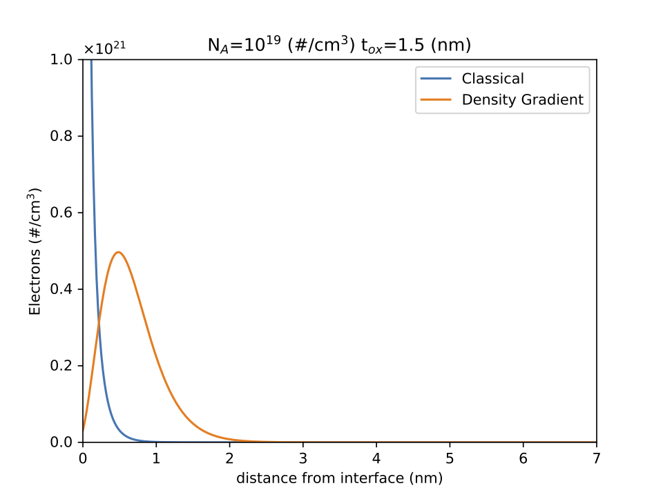
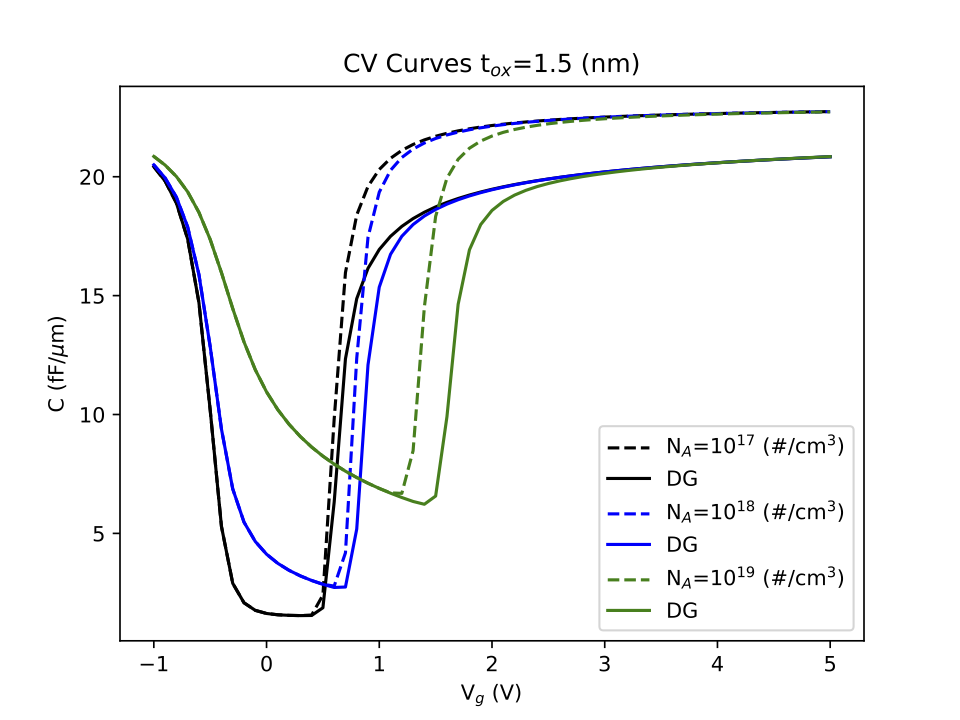
Density Gradient Method
The Density Gradient Method has been implemented as a simulation example for DEVSIM. This method is a quantum mechanical correction for carrier densities near a semiconductor/insulator interface.
The example scripts simulate both a 1D and 2D MOSCAP structure. The scripts generate plots to visualize the results.
It can be downloaded from https://github.com/devsim/devsim_density_gradient.
Semiconductor Device Simulation Using DEVSIM
Semiconductor Device Simulation Using DEVSIM is now available from our site.
Abstract:
DEVSIM is a technology computer aided design (TCAD) simulation software. It is released under an open source license. The software solves user defined partial differential equations (PDEs) on 1D, 2D, and 3D meshes. It is implemented in C++ using custom code and a collection of open source libraries. The Python scripting interface enables users to setup and control their simulations.
In this chapter, we present an overview of the tool. This is followed with a bipolar junction transistor (BJT) design and characterization example. A collection of open source tools were used to create a simulation mesh, and visualize results
The Python scripts for simulation are here:
https://github.com/devsim/devsim_bjt_example
DEVSIM under new open source license
The DEVSIM source code is now released under the Apache License, Version 2.0. It was previously under the LGPL 3.0. The license change is intended to promote adoption of the software and attract new contributors. A brief synopsis of the license is here.
The spirit of the Apache License is also more in line with the license terms packages that DEVSIM relies upon. More information about DEVSIM is available from https://www.devsim.org.
DEVSIM Download
The DEVSIM Open Source TCAD Simulator is now available for download at SourceForge. Packages are available for:
- Mac OS X Mavericks
- Red Hat 6.5
- Ubuntu 12.04
For more information about the project, including source code availability, please visit https://www.devsim.org.
DEVSIM is now Open Source
DEVSIM is now open source. The core engine is licensed under the LGPL 3.0 license, meaning it is available for use in your own software. The project home page is here:
The direct link to the documentation is here:
I hope that this software is useful to the TCAD simulation community. Please let me know if you have any questions about installation or usage of the software.
1D diode junction, part II
In the previous blog post, 1D diode junction I showed some simulation results, here I share some of the actual script for the physics behind this example.
For the poisson equation, the implementation is:
pne = "-ElectronCharge*kahan3(Holes, -Electrons, NetDoping)"
CreateNodeModel(device, region, "PotentialNodeCharge", pne)
CreateNodeModelDerivative(device, region, "PotentialNodeCharge", pne, "Electrons")
CreateNodeModelDerivative(device, region, "PotentialNodeCharge", pne, "Holes")


equation(device=device, region=region, name="PotentialEquation", variable_name="Potential",
node_model="PotentialNodeCharge", edge_model="PotentialEdgeFlux",
time_node_model="", variable_update="log_damp")
where “PotentialEdgeFlux” was defined elsewhere in the script as “Permittivity * ElectricField”. The “kahan3” function is provided to add 3 numbers with additional precision.
For the electron and hole current densities, the Scharfetter-Gummel method is used to calculated the current along each edge connecting the nodes in the mesh. The Bernoulli function, B(x) and its derivative, dBdx(x) are provided in the DEVSIM interpreter
vdiffstr="(Potential@n0 - Potential@n1)/V_t"
CreateEdgeModel(device, region, "vdiff", vdiffstr)
CreateEdgeModel(device, region, "vdiff:Potential@n0", "V_t^(-1)")
CreateEdgeModel(device, region, "vdiff:Potential@n1", "-vdiff:Potential@n0")
CreateEdgeModel(device, region, "Bern01", "B(vdiff)")
CreateEdgeModel(device, region, "Bern01:Potential@n0", "dBdx(vdiff) * vdiff:Potential@n0")
CreateEdgeModel(device, region, "Bern01:Potential@n1", "-Bern01:Potential@n0")
Jn = "ElectronCharge*mu_n*EdgeInverseLength*V_t*kahan3(Electrons@n1*Bern01, Electrons@n1*vdiff, -Electrons@n0*Bern01)"
CreateEdgeModel(device, region, "ElectronCurrent", Jn)
for i in ("Electrons", "Potential", "Holes"):
  CreateEdgeModelDerivatives(device, region, "ElectronCurrent", Jn, i)
In this example, the @n0, and @n1 refers to the variables on each node of the edge. For an edgemodel, “foo”, a derivative with respect to variable on the first node, “bar”, would be “foo:bar@n0”.
For the Shockley Read Hall recombination model, the implementation is:
USRH="(Electrons*Holes - n_i^2)/(taup*(Electrons + n1) + taun*(Holes + p1))"
Gn = "-ElectronCharge * USRH"
Gp = "+ElectronCharge * USRH"
CreateNodeModel(device, region, "USRH", USRH)
CreateNodeModel(device, region, "ElectronGeneration", Gn)
CreateNodeModel(device, region, "HoleGeneration", Gp)
for i in ("Electrons", "Holes"):
  CreateNodeModelDerivative(device, region, "USRH", USRH, i)
  CreateNodeModelDerivative(device, region, "ElectronGeneration", Gn, i)
  CreateNodeModelDerivative(device, region, "HoleGeneration", Gp, i)
The purpose of this post is to describe some of the physics used in the previous example, and show how they are implemented within the DEVSIM software using a scripting interface. Once a set of physical equations has been implemented, it can be placed in modules that can be reused for other simulations.
1D diode junction
It’s always nice when you can get a textbook result from your simulator.
This is the doping profile, and the resulting carrier densities for a forward bias of 0.5 V.

The potential and electric field.

The electron and hole current densities and SRH recombination.

Platform Support
DEVSIM is now supported on Mac OS X. The similarity to Linux and other Unix operating systems made this an easy process. DEVSIM now functions on the following platforms:
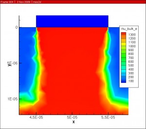
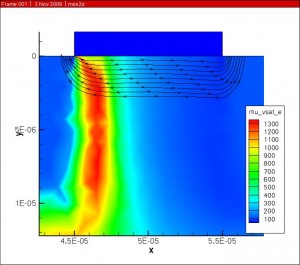
Mobility Modeling
Attached are pictures from a MOSFET simulation operating in the saturation region.
The simulation results are all for the same bias point using the combined electron mobility model.
The Klaassen (Philips) mobility model was implemented for doping and concentration dependence.
The Darwish (Lucent) model was then used to account for the mobility dependence on electric field normal to current flow.
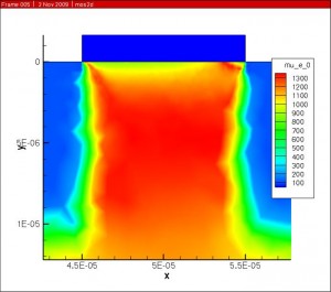
The combined mobility was then scaled by the velocity saturation and is with respect to the electric field parallel to current flow to get the final result.
Future work involves adapting the original Klaassen model so that it agrees with the modifications made in the Darwish paper.
The full implementation of the Klaassen model is presented here, and it tries to follow the original paper. The final mobility is placed on the edge connecting two nodes, and this is done using the geometric mean. Please let me know if you think there are any bugs in the implementation.
set mu_L_e "(mu_max_e * (300 / T)^theta1_e)"

set mu_L_h "(mu_max_h * (300 / T)^theta1_h)"

createNodeModel $device $region mu_L_e "${mu_L_e}"

createNodeModel $device $region mu_L_h "${mu_L_h}"
set mu_e_N "(mu_max_e * mu_max_e / (mu_max_e - mu_min_e) * (T/300)^(3*alpha_1_e - 1.5))"

set mu_h_N "(mu_max_h * mu_max_h / (mu_max_h - mu_min_h) * (T/300)^(3*alpha_1_h - 1.5))"

createNodeModel $device $region mu_e_N "${mu_e_N}"

createNodeModel $device $region mu_h_N "${mu_h_N}"
set mu_e_c "(mu_min_e * mu_max_e / (mu_max_e - mu_min_e)) * (300/T)^(0.5)"

set mu_h_c "(mu_min_h * mu_max_h / (mu_max_h - mu_min_h)) * (300/T)^(0.5)"

createNodeModel $device $region mu_e_c "${mu_e_c}"

createNodeModel $device $region mu_h_c "${mu_h_c}"
set PBH_e "(1.36e20/(Electrons + Holes) * (m_e) * (T/300)^2)"

set PBH_h "(1.36e20/(Electrons + Holes) * (m_h) * (T/300)^2)"

createNodeModel $device $region PBH_e "$PBH_e"

createNodeModelDerivative $device $region PBH_e "$PBH_e" Electrons Holes

createNodeModel $device $region PBH_h "$PBH_h"

createNodeModelDerivative $device $region PBH_h "$PBH_h" Electrons Holes
set Z_D "(1 + 1 / (c_D + (Nref_D / Donors)^2))"

set Z_A "(1 + 1 / (c_A + (Nref_A / Acceptors)^2))"

createNodeModel $device $region Z_D "${Z_D}"

createNodeModel $device $region Z_A "${Z_A}"
set N_D "(Z_D * Donors)"

set N_A "(Z_A * Acceptors)"

createNodeModel $device $region N_D "${N_D}"

createNodeModel $device $region N_A "${N_A}"
set N_e_sc "(N_D + N_A + Holes)"

set N_h_sc "(N_A + N_D + Electrons)"

createNodeModel $device $region N_e_sc "$N_e_sc"

createNodeModelDerivative $device $region N_e_sc "$N_e_sc" Electrons Holes

createNodeModel $device $region N_h_sc "$N_h_sc"

createNodeModelDerivative $device $region N_h_sc "$N_h_sc" Electrons Holes
set PCW_e "(3.97e13 * (1/(Z_D^3 * N_e_sc) * (T/300)^3)^(2/3))"

set PCW_h "(3.97e13 * (1/(Z_A^3 * N_h_sc) * (T/300)^3)^(2/3))"

createNodeModel $device $region PCW_e "$PCW_e"

createNodeModelDerivative $device $region PCW_e "$PCW_e" Electrons Holes

createNodeModel $device $region PCW_h "$PCW_h"

createNodeModelDerivative $device $region PCW_h "$PCW_h" Electrons Holes
set Pe "(1/(f_CW / PCW_e + f_BH/PBH_e))"

set Ph "(1/(f_CW / PCW_h + f_BH/PBH_h))"

createNodeModel $device $region Pe "$Pe"

createNodeModelDerivative $device $region Pe "$Pe" Electrons Holes

createNodeModel $device $region Ph "$Ph"

createNodeModelDerivative $device $region Ph "$Ph" Electrons Holes
set G_Pe "(1 - s1 / (s2 + (1.0/m_e * T/300)^s4 * Pe)^s3 + s5/((m_e * 300/T)^s7*Pe)^s6)"

set G_Ph "(1 - s1 / (s2 + (1.0/m_h * T/300)^s4 * Ph)^s3 + s5/((m_h * 300/T)^s7*Ph)^s6)"

createNodeModel $device $region G_Pe "$G_Pe"

createNodeModelDerivative $device $region G_Pe "$G_Pe" Electrons Holes

createNodeModel $device $region G_Ph "$G_Ph"

createNodeModelDerivative $device $region G_Ph "$G_Ph" Electrons Holes
set F_Pe "((r1 * Pe^r6 + r2 + r3 * m_e/m_h)/(Pe^r6 + r4 + r5 * m_e/m_h))"

set F_Ph "((r1 * Ph^r6 + r2 + r3 * m_h/m_e)/(Ph^r6 + r4 + r5 * m_h/m_e))"

createNodeModel $device $region F_Pe "$F_Pe"

createNodeModelDerivative $device $region F_Pe "$F_Pe" Electrons Holes

createNodeModel $device $region F_Ph "$F_Ph"

createNodeModelDerivative $device $region F_Ph "$F_Ph" Electrons Holes
set N_e_sc_eff "(N_D + G_Pe * N_A + Holes / F_Pe)"

set N_h_sc_eff "(N_A + G_Ph * N_D + Electrons / F_Ph)"

createNodeModel $device $region N_e_sc_eff "$N_e_sc_eff"

createNodeModelDerivative $device $region N_e_sc_eff "$N_e_sc_eff" Electrons Holes

createNodeModel $device $region N_h_sc_eff "$N_h_sc_eff"

createNodeModelDerivative $device $region N_h_sc_eff "$N_h_sc_eff" Electrons Holes
set mu_e_D_A_h "mu_e_N * N_e_sc/N_e_sc_eff * (Nref_1_e / N_e_sc)^alpha_1_e + mu_e_c * ((Electrons + Holes)/N_e_sc_eff)"

set mu_h_D_A_e "mu_h_N * N_h_sc/N_h_sc_eff * (Nref_1_h / N_h_sc)^alpha_1_h + mu_h_c * ((Electrons + Holes)/N_h_sc_eff)"

createNodeModel $device $region mu_e_D_A_h "${mu_e_D_A_h}"

createNodeModelDerivative $device $region mu_e_D_A_h "${mu_e_D_A_h}" Electrons Holes

createNodeModel $device $region mu_h_D_A_e "${mu_h_D_A_e}"

createNodeModelDerivative $device $region mu_h_D_A_e "${mu_h_D_A_e}" Electrons Holes
set mu_bulk_e_Node "mu_e_D_A_h * mu_L_e / (mu_e_D_A_h + mu_L_e)"

createNodeModel $device $region mu_bulk_e_Node "${mu_bulk_e_Node}"

createNodeModelDerivative $device $region mu_bulk_e_Node "${mu_bulk_e_Node}" Electrons Holes
set mu_bulk_h_Node "mu_h_D_A_e * mu_L_h / (mu_h_D_A_e + mu_L_h)"

createNodeModel $device $region mu_bulk_h_Node "${mu_bulk_h_Node}"

createNodeModelDerivative $device $region mu_bulk_h_Node "${mu_bulk_h_Node}" Electrons Holes
createGeometricMean $device $region mu_bulk_e_Node mu_bulk_e

createGeometricMeanDerivative $device $region mu_bulk_e_Node mu_bulk_e Electrons Holes

createGeometricMean $device $region mu_bulk_h_Node mu_bulk_h

createGeometricMeanDerivative $device $region mu_bulk_h_Node mu_bulk_h Electrons Holes