Category Archives: TCAD

DEVSIM is now Open Source

DEVSIM is now open source. The core engine is licensed under the LGPL 3.0 license, meaning it is available for use in your own software. The project home page is here:

https://devsim.org

The direct link to the documentation is here:

https://devsim.org/manual

I hope that this software is useful to the TCAD simulation community. Please let me know if you have any questions about installation or usage of the software.

1D diode junction, part II

In the previous blog post, 1D diode junction I showed some simulation results, here I share some of the actual script for the physics behind this example.

For the poisson equation, the implementation is:

pne = "-ElectronCharge*kahan3(Holes, -Electrons, NetDoping)"
CreateNodeModel(device, region, "PotentialNodeCharge", pne)
CreateNodeModelDerivative(device, region, "PotentialNodeCharge", pne, "Electrons")
CreateNodeModelDerivative(device, region, "PotentialNodeCharge", pne, "Holes")


equation(device=device, region=region, name="PotentialEquation", variable_name="Potential",
node_model="PotentialNodeCharge", edge_model="PotentialEdgeFlux",
time_node_model="", variable_update="log_damp")

where “PotentialEdgeFlux” was defined elsewhere in the script as “Permittivity * ElectricField”. The “kahan3” function is provided to add 3 numbers with additional precision.

For the electron and hole current densities, the Scharfetter-Gummel method is used to calculated the current along each edge connecting the nodes in the mesh. The Bernoulli function, B(x) and its derivative, dBdx(x) are provided in the DEVSIM interpreter

vdiffstr="(Potential@n0 - Potential@n1)/V_t"
CreateEdgeModel(device, region, "vdiff", vdiffstr)
CreateEdgeModel(device, region, "vdiff:Potential@n0", "V_t^(-1)")
CreateEdgeModel(device, region, "vdiff:Potential@n1", "-vdiff:Potential@n0")
CreateEdgeModel(device, region, "Bern01", "B(vdiff)")
CreateEdgeModel(device, region, "Bern01:Potential@n0", "dBdx(vdiff) * vdiff:Potential@n0")
CreateEdgeModel(device, region, "Bern01:Potential@n1", "-Bern01:Potential@n0")
Jn = "ElectronCharge*mu_n*EdgeInverseLength*V_t*kahan3(Electrons@n1*Bern01, Electrons@n1*vdiff, -Electrons@n0*Bern01)"
CreateEdgeModel(device, region, "ElectronCurrent", Jn)
for i in ("Electrons", "Potential", "Holes"):
  CreateEdgeModelDerivatives(device, region, "ElectronCurrent", Jn, i)

In this example, the @n0, and @n1 refers to the variables on each node of the edge. For an edgemodel, “foo”, a derivative with respect to variable on the first node, “bar”, would be “foo:bar@n0”.

For the Shockley Read Hall recombination model, the implementation is:

USRH="(Electrons*Holes - n_i^2)/(taup*(Electrons + n1) + taun*(Holes + p1))"
Gn = "-ElectronCharge * USRH"
Gp = "+ElectronCharge * USRH"
CreateNodeModel(device, region, "USRH", USRH)
CreateNodeModel(device, region, "ElectronGeneration", Gn)
CreateNodeModel(device, region, "HoleGeneration", Gp)
for i in ("Electrons", "Holes"):
  CreateNodeModelDerivative(device, region, "USRH", USRH, i)
  CreateNodeModelDerivative(device, region, "ElectronGeneration", Gn, i)
  CreateNodeModelDerivative(device, region, "HoleGeneration", Gp, i)

The purpose of this post is to describe some of the physics used in the previous example, and show how they are implemented within the DEVSIM software using a scripting interface. Once a set of physical equations has been implemented, it can be placed in modules that can be reused for other simulations.
1D diode junction

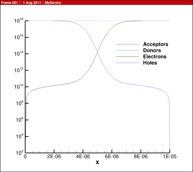
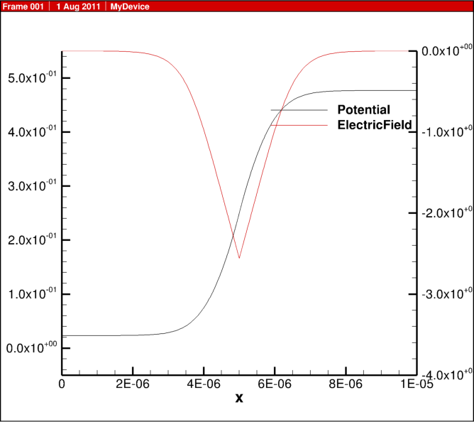
It’s always nice when you can get a textbook result from your simulator.

This is the doping profile, and the resulting carrier densities for a forward bias of 0.5 V.

The potential and electric field.

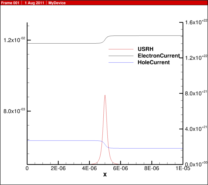
The electron and hole current densities and SRH recombination.

Platform Support

DEVSIM is now supported on Mac OS X. The similarity to Linux and other Unix operating systems made this an easy process. DEVSIM now functions on the following platforms:

  • Linux (32, 64 bit)
  • Mac OS X (32, 64 bit)
  • Windows (32 bit)
  • Mobility Modeling

    Attached are pictures from a MOSFET simulation operating in the saturation region.

    The simulation results are all for the same bias point using the combined electron mobility model.

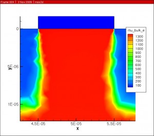
    The Klaassen (Philips) mobility model was implemented for doping and concentration dependence.

    bulk_e

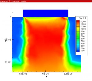
    The Darwish (Lucent) model was then used to account for the mobility dependence on electric field normal to current flow.

    mu_e_0

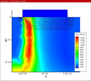
    The combined mobility was then scaled by the velocity saturation and is with respect to the electric field parallel to current flow to get the final result.

    vsat_e

    Future work involves adapting the original Klaassen model so that it agrees with the modifications made in the Darwish paper.

    The full implementation of the Klaassen model is presented here, and it tries to follow the original paper. The final mobility is placed on the edge connecting two nodes, and this is done using the geometric mean. Please let me know if you think there are any bugs in the implementation.


    set mu_L_e "(mu_max_e * (300 / T)^theta1_e)"
    set mu_L_h "(mu_max_h * (300 / T)^theta1_h)"
    createNodeModel $device $region mu_L_e "${mu_L_e}"
    createNodeModel $device $region mu_L_h "${mu_L_h}"


    set mu_e_N "(mu_max_e * mu_max_e / (mu_max_e - mu_min_e) * (T/300)^(3*alpha_1_e - 1.5))"
    set mu_h_N "(mu_max_h * mu_max_h / (mu_max_h - mu_min_h) * (T/300)^(3*alpha_1_h - 1.5))"
    createNodeModel $device $region mu_e_N "${mu_e_N}"
    createNodeModel $device $region mu_h_N "${mu_h_N}"


    set mu_e_c "(mu_min_e * mu_max_e / (mu_max_e - mu_min_e)) * (300/T)^(0.5)"
    set mu_h_c "(mu_min_h * mu_max_h / (mu_max_h - mu_min_h)) * (300/T)^(0.5)"
    createNodeModel $device $region mu_e_c "${mu_e_c}"
    createNodeModel $device $region mu_h_c "${mu_h_c}"


    set PBH_e "(1.36e20/(Electrons + Holes) * (m_e) * (T/300)^2)"
    set PBH_h "(1.36e20/(Electrons + Holes) * (m_h) * (T/300)^2)"
    createNodeModel $device $region PBH_e "$PBH_e"
    createNodeModelDerivative $device $region PBH_e "$PBH_e" Electrons Holes
    createNodeModel $device $region PBH_h "$PBH_h"
    createNodeModelDerivative $device $region PBH_h "$PBH_h" Electrons Holes


    set Z_D "(1 + 1 / (c_D + (Nref_D / Donors)^2))"
    set Z_A "(1 + 1 / (c_A + (Nref_A / Acceptors)^2))"
    createNodeModel $device $region Z_D "${Z_D}"
    createNodeModel $device $region Z_A "${Z_A}"


    set N_D "(Z_D * Donors)"
    set N_A "(Z_A * Acceptors)"
    createNodeModel $device $region N_D "${N_D}"
    createNodeModel $device $region N_A "${N_A}"


    set N_e_sc "(N_D + N_A + Holes)"
    set N_h_sc "(N_A + N_D + Electrons)"
    createNodeModel $device $region N_e_sc "$N_e_sc"
    createNodeModelDerivative $device $region N_e_sc "$N_e_sc" Electrons Holes
    createNodeModel $device $region N_h_sc "$N_h_sc"
    createNodeModelDerivative $device $region N_h_sc "$N_h_sc" Electrons Holes


    set PCW_e "(3.97e13 * (1/(Z_D^3 * N_e_sc) * (T/300)^3)^(2/3))"
    set PCW_h "(3.97e13 * (1/(Z_A^3 * N_h_sc) * (T/300)^3)^(2/3))"
    createNodeModel $device $region PCW_e "$PCW_e"
    createNodeModelDerivative $device $region PCW_e "$PCW_e" Electrons Holes
    createNodeModel $device $region PCW_h "$PCW_h"
    createNodeModelDerivative $device $region PCW_h "$PCW_h" Electrons Holes


    set Pe "(1/(f_CW / PCW_e + f_BH/PBH_e))"
    set Ph "(1/(f_CW / PCW_h + f_BH/PBH_h))"
    createNodeModel $device $region Pe "$Pe"
    createNodeModelDerivative $device $region Pe "$Pe" Electrons Holes
    createNodeModel $device $region Ph "$Ph"
    createNodeModelDerivative $device $region Ph "$Ph" Electrons Holes


    set G_Pe "(1 - s1 / (s2 + (1.0/m_e * T/300)^s4 * Pe)^s3 + s5/((m_e * 300/T)^s7*Pe)^s6)"
    set G_Ph "(1 - s1 / (s2 + (1.0/m_h * T/300)^s4 * Ph)^s3 + s5/((m_h * 300/T)^s7*Ph)^s6)"
    createNodeModel $device $region G_Pe "$G_Pe"
    createNodeModelDerivative $device $region G_Pe "$G_Pe" Electrons Holes
    createNodeModel $device $region G_Ph "$G_Ph"
    createNodeModelDerivative $device $region G_Ph "$G_Ph" Electrons Holes


    set F_Pe "((r1 * Pe^r6 + r2 + r3 * m_e/m_h)/(Pe^r6 + r4 + r5 * m_e/m_h))"
    set F_Ph "((r1 * Ph^r6 + r2 + r3 * m_h/m_e)/(Ph^r6 + r4 + r5 * m_h/m_e))"
    createNodeModel $device $region F_Pe "$F_Pe"
    createNodeModelDerivative $device $region F_Pe "$F_Pe" Electrons Holes
    createNodeModel $device $region F_Ph "$F_Ph"
    createNodeModelDerivative $device $region F_Ph "$F_Ph" Electrons Holes


    set N_e_sc_eff "(N_D + G_Pe * N_A + Holes / F_Pe)"
    set N_h_sc_eff "(N_A + G_Ph * N_D + Electrons / F_Ph)"
    createNodeModel $device $region N_e_sc_eff "$N_e_sc_eff"
    createNodeModelDerivative $device $region N_e_sc_eff "$N_e_sc_eff" Electrons Holes
    createNodeModel $device $region N_h_sc_eff "$N_h_sc_eff"
    createNodeModelDerivative $device $region N_h_sc_eff "$N_h_sc_eff" Electrons Holes


    set mu_e_D_A_h "mu_e_N * N_e_sc/N_e_sc_eff * (Nref_1_e / N_e_sc)^alpha_1_e + mu_e_c * ((Electrons + Holes)/N_e_sc_eff)"
    set mu_h_D_A_e "mu_h_N * N_h_sc/N_h_sc_eff * (Nref_1_h / N_h_sc)^alpha_1_h + mu_h_c * ((Electrons + Holes)/N_h_sc_eff)"
    createNodeModel $device $region mu_e_D_A_h "${mu_e_D_A_h}"
    createNodeModelDerivative $device $region mu_e_D_A_h "${mu_e_D_A_h}" Electrons Holes
    createNodeModel $device $region mu_h_D_A_e "${mu_h_D_A_e}"
    createNodeModelDerivative $device $region mu_h_D_A_e "${mu_h_D_A_e}" Electrons Holes


    set mu_bulk_e_Node "mu_e_D_A_h * mu_L_e / (mu_e_D_A_h + mu_L_e)"
    createNodeModel $device $region mu_bulk_e_Node "${mu_bulk_e_Node}"
    createNodeModelDerivative $device $region mu_bulk_e_Node "${mu_bulk_e_Node}" Electrons Holes


    set mu_bulk_h_Node "mu_h_D_A_e * mu_L_h / (mu_h_D_A_e + mu_L_h)"
    createNodeModel $device $region mu_bulk_h_Node "${mu_bulk_h_Node}"
    createNodeModelDerivative $device $region mu_bulk_h_Node "${mu_bulk_h_Node}" Electrons Holes


    createGeometricMean $device $region mu_bulk_e_Node mu_bulk_e
    createGeometricMeanDerivative $device $region mu_bulk_e_Node mu_bulk_e Electrons Holes
    createGeometricMean $device $region mu_bulk_h_Node mu_bulk_h
    createGeometricMeanDerivative $device $region mu_bulk_h_Node mu_bulk_h Electrons Holes

    Biosensor Applications in DEVSIM (Part II)

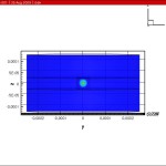
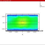
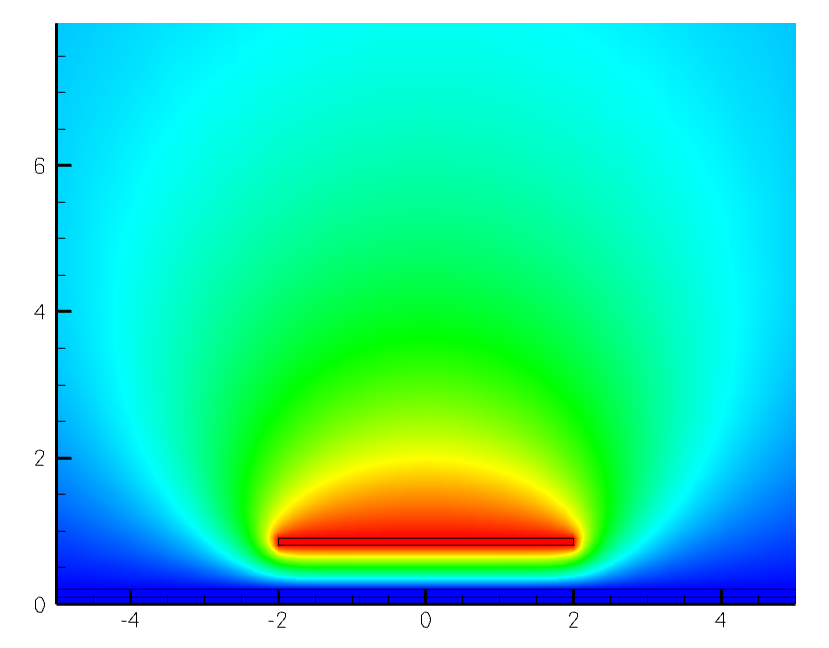
    As a follow up to the previous post, here are the results when 3d versions of the structures were created. The active areas are in the center of the device, and the rest of the device are translucent.

    Biosensor Applications in DEVSIM

    I became interested in replicating the results in this paper:
    Y. Liu, J. Sauer, and R. Dutton, “Effect of electro-diffusion current flow on electrostatic screening in aqueous pores,” Journal of Applied Physics, Vol. 103, p.084701, 2008

    which Dr. Liu provides on his website here:
    http://www-tcad.stanford.edu/~yangliu/

    The two plots in this post reflect the effect of a charged macro molecule (e.g. DNA) under biased and unbiased conditions in the structure. The structure has contacts at the top and bottom. The plots for a bias of 0 and 7 volts are included in this post. The plots show the potential difference when the charged macro molecule is present and not present in the aqueous pore to the center left of the picture. More information about the significance of the result may be found in Dr. Liu’s paper.

    In order to replicate Dr. Liu’s results, the cylindrical coordinate system was implemented in DEVSIM. The device is cylindrical and the structure is wrapped around the left vertical axis. The PDE’s for the potential and flux densities were implemented in a fashion similar to the standard drift diffusion formalism for TCAD simulation.

    Porting DEVSIM to Windows

    While our primary development platform is 64-bit Linux, work is in process to get DEVSIM working on 32-bit Windows. It has been challenging, but thankfully the porting process has become easier as compiler vendors have become more standards compliant. It is especially nice that the majority of the third party components of our software already support Windows and Unix-like platforms.

    One of the benefits of porting with a new compiler has been to identify code which is not necessarily portable across computer architectures, or entirely C++ standards compliant. This effort has even enabled us to find a few minor defects in our implementation.

    I am happy to report that we have a functioning build on Windows, and thorough regression testing is in progress.

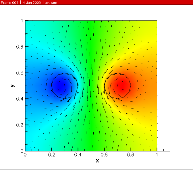
    Solving for magnetic fields in DEVSIM.

    This past week I’ve been experimenting with solving magnetic field problems. Here is my first result. Two wires are in the center of the figure with current flowing in opposite directions. The solution variable is the magnetic vector potential, A, and is shown in the color gradient. The arrows are the magnetic field, B, which is post processed from the solution. In turns out this post processing is similar to finding the vector impedance field used in noise analysis.

    twowire1