DEVSIM is now supported on Mac OS X. The similarity to Linux and other Unix operating systems made this an easy process. DEVSIM now functions on the following platforms:
Mobility Modeling
Attached are pictures from a MOSFET simulation operating in the saturation region.
The simulation results are all for the same bias point using the combined electron mobility model.
The Klaassen (Philips) mobility model was implemented for doping and concentration dependence.
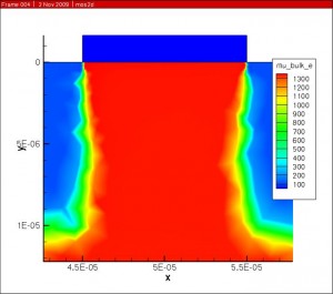
The Darwish (Lucent) model was then used to account for the mobility dependence on electric field normal to current flow.
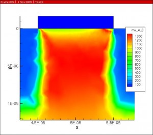
The combined mobility was then scaled by the velocity saturation and is with respect to the electric field parallel to current flow to get the final result.
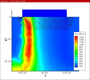
Future work involves adapting the original Klaassen model so that it agrees with the modifications made in the Darwish paper.
The full implementation of the Klaassen model is presented here, and it tries to follow the original paper. The final mobility is placed on the edge connecting two nodes, and this is done using the geometric mean. Please let me know if you think there are any bugs in the implementation.
set mu_L_e "(mu_max_e * (300 / T)^theta1_e)"

set mu_L_h "(mu_max_h * (300 / T)^theta1_h)"

createNodeModel $device $region mu_L_e "${mu_L_e}"

createNodeModel $device $region mu_L_h "${mu_L_h}"
set mu_e_N "(mu_max_e * mu_max_e / (mu_max_e - mu_min_e) * (T/300)^(3*alpha_1_e - 1.5))"

set mu_h_N "(mu_max_h * mu_max_h / (mu_max_h - mu_min_h) * (T/300)^(3*alpha_1_h - 1.5))"

createNodeModel $device $region mu_e_N "${mu_e_N}"

createNodeModel $device $region mu_h_N "${mu_h_N}"
set mu_e_c "(mu_min_e * mu_max_e / (mu_max_e - mu_min_e)) * (300/T)^(0.5)"

set mu_h_c "(mu_min_h * mu_max_h / (mu_max_h - mu_min_h)) * (300/T)^(0.5)"

createNodeModel $device $region mu_e_c "${mu_e_c}"

createNodeModel $device $region mu_h_c "${mu_h_c}"
set PBH_e "(1.36e20/(Electrons + Holes) * (m_e) * (T/300)^2)"

set PBH_h "(1.36e20/(Electrons + Holes) * (m_h) * (T/300)^2)"

createNodeModel $device $region PBH_e "$PBH_e"

createNodeModelDerivative $device $region PBH_e "$PBH_e" Electrons Holes

createNodeModel $device $region PBH_h "$PBH_h"

createNodeModelDerivative $device $region PBH_h "$PBH_h" Electrons Holes
set Z_D "(1 + 1 / (c_D + (Nref_D / Donors)^2))"

set Z_A "(1 + 1 / (c_A + (Nref_A / Acceptors)^2))"

createNodeModel $device $region Z_D "${Z_D}"

createNodeModel $device $region Z_A "${Z_A}"
set N_D "(Z_D * Donors)"

set N_A "(Z_A * Acceptors)"

createNodeModel $device $region N_D "${N_D}"

createNodeModel $device $region N_A "${N_A}"
set N_e_sc "(N_D + N_A + Holes)"

set N_h_sc "(N_A + N_D + Electrons)"

createNodeModel $device $region N_e_sc "$N_e_sc"

createNodeModelDerivative $device $region N_e_sc "$N_e_sc" Electrons Holes

createNodeModel $device $region N_h_sc "$N_h_sc"

createNodeModelDerivative $device $region N_h_sc "$N_h_sc" Electrons Holes
set PCW_e "(3.97e13 * (1/(Z_D^3 * N_e_sc) * (T/300)^3)^(2/3))"

set PCW_h "(3.97e13 * (1/(Z_A^3 * N_h_sc) * (T/300)^3)^(2/3))"

createNodeModel $device $region PCW_e "$PCW_e"

createNodeModelDerivative $device $region PCW_e "$PCW_e" Electrons Holes

createNodeModel $device $region PCW_h "$PCW_h"

createNodeModelDerivative $device $region PCW_h "$PCW_h" Electrons Holes
set Pe "(1/(f_CW / PCW_e + f_BH/PBH_e))"

set Ph "(1/(f_CW / PCW_h + f_BH/PBH_h))"

createNodeModel $device $region Pe "$Pe"

createNodeModelDerivative $device $region Pe "$Pe" Electrons Holes

createNodeModel $device $region Ph "$Ph"

createNodeModelDerivative $device $region Ph "$Ph" Electrons Holes
set G_Pe "(1 - s1 / (s2 + (1.0/m_e * T/300)^s4 * Pe)^s3 + s5/((m_e * 300/T)^s7*Pe)^s6)"

set G_Ph "(1 - s1 / (s2 + (1.0/m_h * T/300)^s4 * Ph)^s3 + s5/((m_h * 300/T)^s7*Ph)^s6)"

createNodeModel $device $region G_Pe "$G_Pe"

createNodeModelDerivative $device $region G_Pe "$G_Pe" Electrons Holes

createNodeModel $device $region G_Ph "$G_Ph"

createNodeModelDerivative $device $region G_Ph "$G_Ph" Electrons Holes
set F_Pe "((r1 * Pe^r6 + r2 + r3 * m_e/m_h)/(Pe^r6 + r4 + r5 * m_e/m_h))"

set F_Ph "((r1 * Ph^r6 + r2 + r3 * m_h/m_e)/(Ph^r6 + r4 + r5 * m_h/m_e))"

createNodeModel $device $region F_Pe "$F_Pe"

createNodeModelDerivative $device $region F_Pe "$F_Pe" Electrons Holes

createNodeModel $device $region F_Ph "$F_Ph"

createNodeModelDerivative $device $region F_Ph "$F_Ph" Electrons Holes
set N_e_sc_eff "(N_D + G_Pe * N_A + Holes / F_Pe)"

set N_h_sc_eff "(N_A + G_Ph * N_D + Electrons / F_Ph)"

createNodeModel $device $region N_e_sc_eff "$N_e_sc_eff"

createNodeModelDerivative $device $region N_e_sc_eff "$N_e_sc_eff" Electrons Holes

createNodeModel $device $region N_h_sc_eff "$N_h_sc_eff"

createNodeModelDerivative $device $region N_h_sc_eff "$N_h_sc_eff" Electrons Holes
set mu_e_D_A_h "mu_e_N * N_e_sc/N_e_sc_eff * (Nref_1_e / N_e_sc)^alpha_1_e + mu_e_c * ((Electrons + Holes)/N_e_sc_eff)"

set mu_h_D_A_e "mu_h_N * N_h_sc/N_h_sc_eff * (Nref_1_h / N_h_sc)^alpha_1_h + mu_h_c * ((Electrons + Holes)/N_h_sc_eff)"

createNodeModel $device $region mu_e_D_A_h "${mu_e_D_A_h}"

createNodeModelDerivative $device $region mu_e_D_A_h "${mu_e_D_A_h}" Electrons Holes

createNodeModel $device $region mu_h_D_A_e "${mu_h_D_A_e}"

createNodeModelDerivative $device $region mu_h_D_A_e "${mu_h_D_A_e}" Electrons Holes
set mu_bulk_e_Node "mu_e_D_A_h * mu_L_e / (mu_e_D_A_h + mu_L_e)"

createNodeModel $device $region mu_bulk_e_Node "${mu_bulk_e_Node}"

createNodeModelDerivative $device $region mu_bulk_e_Node "${mu_bulk_e_Node}" Electrons Holes
set mu_bulk_h_Node "mu_h_D_A_e * mu_L_h / (mu_h_D_A_e + mu_L_h)"

createNodeModel $device $region mu_bulk_h_Node "${mu_bulk_h_Node}"

createNodeModelDerivative $device $region mu_bulk_h_Node "${mu_bulk_h_Node}" Electrons Holes
createGeometricMean $device $region mu_bulk_e_Node mu_bulk_e

createGeometricMeanDerivative $device $region mu_bulk_e_Node mu_bulk_e Electrons Holes

createGeometricMean $device $region mu_bulk_h_Node mu_bulk_h

createGeometricMeanDerivative $device $region mu_bulk_h_Node mu_bulk_h Electrons Holes
SISPAD 2009
I am glad I went to this year’s SISPAD 2009. There were many fascinating papers and I had the opportunity to meet with several researchers doing some interesting work.
There were many papers using Non-Equilibrium Green’s Functions~(NEGF). I’ve always had difficulty in understanding the approach, but Dipanjan Basu from the University of Texas at Austin gave me one of the best explanations.
NEGF, Monte Carlo (MC), and Spherical Harmonic Expansions of the Bolztmann Equations (SHE) seemed to be popular simulation methods for nano-devices. The molecular dynamics simulations of Dr. K.-R. Lee of KIST were quite impressive showing the interactions of Al and Co atoms.
I am glad to see device simulation using continuum PDE simulation is still considered important. There is also an exciting application of this method and MC to bio-sensor applications.
Dr. Ancona gave an interesting talk using Density Gradient theory to model Sb-based PFET’s. He used the COMSOL multiphysics package to do his simulations. This piqued my interest as I am writing a generalized PDE solver of my own. Being a finite element package (FE), it was surprising he was able to overcome the issues with current density calculations without using Scharfetter Gummel (SG).
Aryan Afzalian also had an interesting paper where he used COMSOL as part of his NEGF simulation method.
One of the most entertaining speakers was Professor Wachutka from TU Munich. He had a fascinating discussion of the importance power devices, and the interesting effects which need to be modeled using TCAD.
In addition to Synopsys, TCAD International and Global TCAD Solutions were TCAD companies sponsoring the event. It is good to see that there is room in the TCAD simulation market.
I was also appreciative that Clemens Heitzinger (University of Vienna) and Yang Liu (Stanford) were there to discuss bio-sensors. Greg Rollins (Synopsys) and Valery Axelrad (SEQUOIA Design Systems) were also kind enough to share their insight into TCAD device simulation issues.
Many thanks to the SISPAD organizers for an excellent conference.
Biosensor Applications in DEVSIM (Part II)
As a follow up to the previous post, here are the results when 3d versions of the structures were created. The active areas are in the center of the device, and the rest of the device are translucent.
Biosensor Applications in DEVSIM
I became interested in replicating the results in this paper:
Y. Liu, J. Sauer, and R. Dutton, “Effect of electro-diffusion current flow on electrostatic screening in aqueous pores,” Journal of Applied Physics, Vol. 103, p.084701, 2008
which Dr. Liu provides on his website here:
http://www-tcad.stanford.edu/~yangliu/
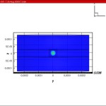
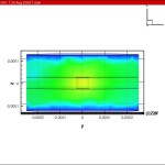
The two plots in this post reflect the effect of a charged macro molecule (e.g. DNA) under biased and unbiased conditions in the structure. The structure has contacts at the top and bottom. The plots for a bias of 0 and 7 volts are included in this post. The plots show the potential difference when the charged macro molecule is present and not present in the aqueous pore to the center left of the picture. More information about the significance of the result may be found in Dr. Liu’s paper.
In order to replicate Dr. Liu’s results, the cylindrical coordinate system was implemented in DEVSIM. The device is cylindrical and the structure is wrapped around the left vertical axis. The PDE’s for the potential and flux densities were implemented in a fashion similar to the standard drift diffusion formalism for TCAD simulation.
- ve0
- ve7
Porting DEVSIM to Windows
While our primary development platform is 64-bit Linux, work is in process to get DEVSIM working on 32-bit Windows. It has been challenging, but thankfully the porting process has become easier as compiler vendors have become more standards compliant. It is especially nice that the majority of the third party components of our software already support Windows and Unix-like platforms.
One of the benefits of porting with a new compiler has been to identify code which is not necessarily portable across computer architectures, or entirely C++ standards compliant. This effort has even enabled us to find a few minor defects in our implementation.
I am happy to report that we have a functioning build on Windows, and thorough regression testing is in progress.
Capacitance Simulation
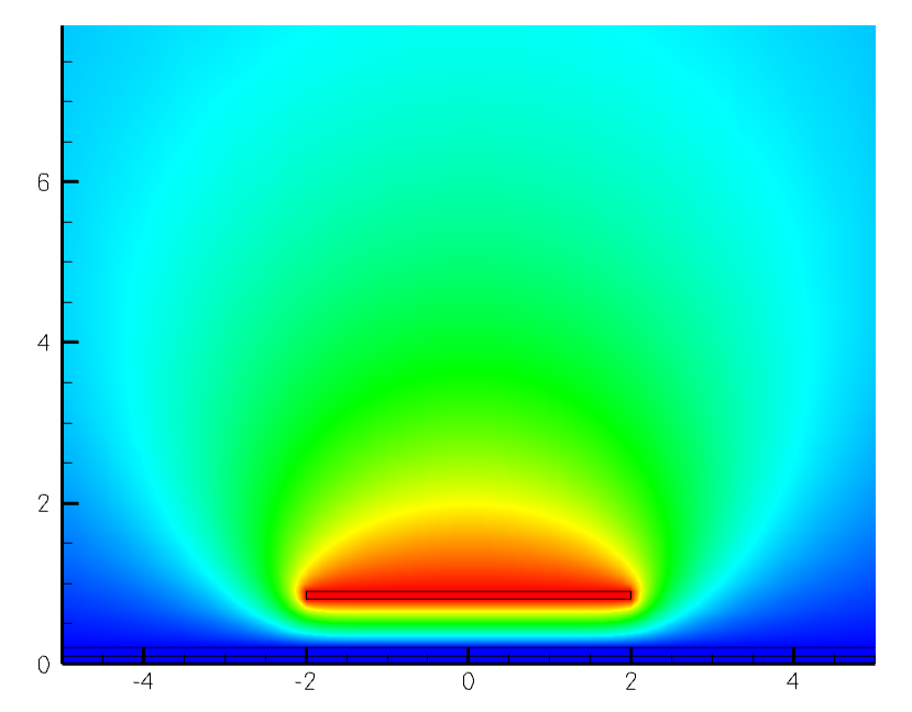
This is a simulation of a single conductor above a ground plane. The simulation window is actually much larger to ensure proper boundary conditions.
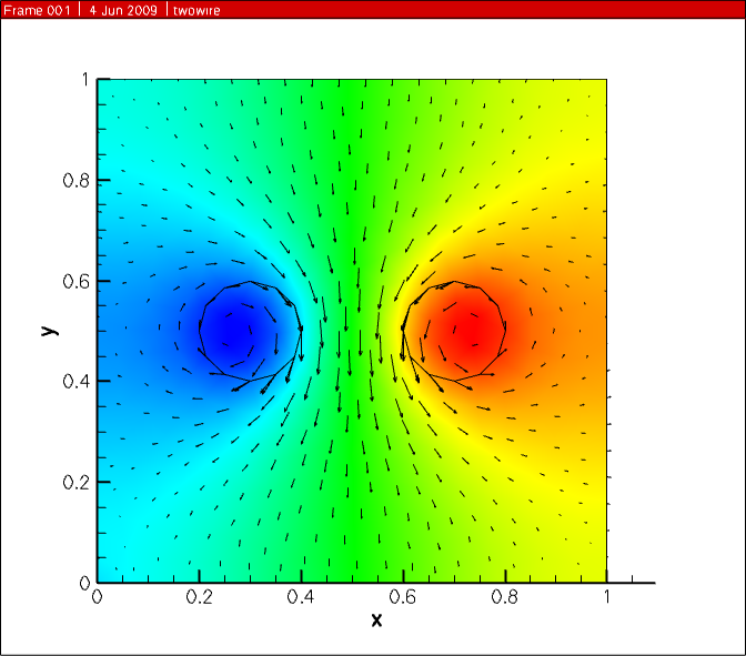
Solving for magnetic fields in DEVSIM.
This past week I’ve been experimenting with solving magnetic field problems. Here is my first result. Two wires are in the center of the figure with current flowing in opposite directions. The solution variable is the magnetic vector potential, A, and is shown in the color gradient. The arrows are the magnetic field, B, which is post processed from the solution. In turns out this post processing is similar to finding the vector impedance field used in noise analysis.
Sensitivity Analysis White Paper
A new white paper concerning sensitivity analysis is available here:
TCAD Sensitivity Analysis for Device Optimization
New White Paper
I have uploaded a white paper to the website. It discusses some of the concepts behind DEVSIM.
Symbolic Model Evaluation for TCAD Device Simulation
